Case Study

Inventory Forecasting Using Machine Learning

Improving inventory visibility in a system shaped by uncertainty, delayed information, and imperfect signals.

30 / 60 / 90

Day forecasting horizons explored within the planning cycle

Weekly

Forecast generation cadence using the most recent available data

Monthly

Model retraining cycle to absorb new information over time

Hybrid

Modelling strategy combining classification, regression, and temporal features

Project context

In large supply chain environments, inventory planning is typically shaped by a combination of system-generated forecasts and manual adjustments. These approaches tend to work reasonably well when demand and supply remain relatively stable, but their limitations become more visible as variability increases, particularly when there are delays in order booking, uncertainty in delivery timelines, or gaps in the information available to the planning process.

This work was part of a broader effort to explore whether machine learning could improve inventory forecasting for a global supply hub. The objective was not to replace existing planning systems, but to complement them with a more structured and data-driven perspective on how inventory might evolve over the next thirty, sixty, and ninety days.

As the work progressed, it became clear that the problem could not be treated simply as a point prediction task. It required a better understanding of how events unfold over time, which naturally led to the exploration of both traditional machine learning approaches and models intended to capture temporal dependencies.

Problem definition

The forecasting challenge was not only about predicting future inventory positions, but also about accounting for delays and information gaps that distorted the picture available to planners. Inventory outcomes depended on what had already happened, what had been booked into the system, and what had not yet become visible in the data.

This meant the forecasting task sat somewhere between demand prediction, delay estimation, and operational decision support. The real question was whether a machine learning-based approach could produce a more stable and useful view than the planning baseline.

Constraints

Long-term visibility was limited because a substantial share of orders appeared late in the cycle.
Delay patterns existed in the data, but the underlying causes were not always explicitly captured.
Forecasts needed to operate across many materials rather than a small controlled subset.
The work had to move beyond notebook experimentation toward a pipeline that could be run more consistently.

Approach

The work followed an intentionally iterative approach. Rather than committing too early to a single modelling strategy, multiple techniques were explored to understand what the data could realistically support.

The initial direction focused on modelling individual orders. The idea was to predict whether an order would be delayed and then estimate the extent of that delay, after which those predictions could be aggregated into an overall inventory forecast. In practice, this approach did not perform well. The signals at the individual order level were too noisy, and the models struggled to generalise in a meaningful way.

The modelling strategy was then refined by shifting from order-level prediction to material-level aggregation. This reduced variability and allowed more stable patterns to emerge. At the same time, the modelling logic was decomposed into two related tasks. One component estimated whether delays were likely, while another estimated their timing.

A significant portion of the work was directed toward feature engineering. Rather than relying only on raw historical values, the system incorporated lagged observations, rolling statistics, and time-based signals. This made it possible to capture important temporal behaviour without depending entirely on deep learning approaches.

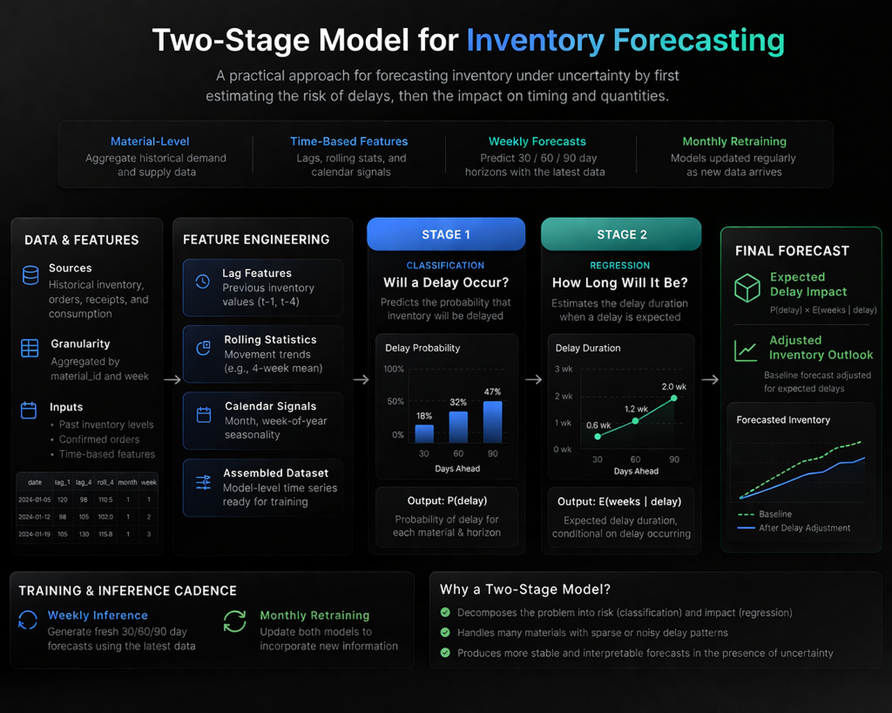
System architecture

The forecasting system follows a two-stage modelling approach. First, a classification model estimates the likelihood of delay. This is followed by a regression model that estimates the expected duration of delay. These outputs are then combined to adjust the baseline inventory forecast.

Two-stage inventory forecasting model architecture

Model exploration

Several families of models were explored over the course of the work. The aim was not to test complexity for its own sake, but to understand which methods were most compatible with the structure and limitations of the data.

Linear and regularised regression approaches were explored as simple baselines.
Tree-based methods such as Random Forest and Gradient Boosting were evaluated for their ability to handle non-linear behaviour.
Classification models were tested for delay prediction, while regression models were used to estimate timing effects.
Sequence-based models such as LSTMs were explored to capture temporal dependencies more explicitly.

What I built

The work moved beyond isolated experimentation toward a more repeatable forecasting workflow. Data extraction and transformation pipelines were built to prepare material-level time series inputs, generate the required lag and rolling features, and support regular model retraining.

The system was structured to produce recurring forecasts on a weekly basis while allowing monthly retraining as new information arrived. Backtesting was used to compare outputs against historical outcomes and against the planning baseline, helping clarify where the machine learning approach added value and where it remained constrained by data visibility.

Illustrative implementation snippets

The original enterprise implementation is not shared publicly. The examples below are simplified representations of the modelling logic, included to show the structure of the work rather than the exact production code.

Material-level feature engineering

def create_features(df):
    df = df.sort_values(["material_id", "date"])
    df["lag_1"] = df.groupby("material_id")["quantity"].shift(1)
    df["lag_4"] = df.groupby("material_id")["quantity"].shift(4)
    df["rolling_mean_4"] = (
        df.groupby("material_id")["quantity"]
          .rolling(window=4)
          .mean()
          .reset_index(level=0, drop=True)
    )
    df["month"] = df["date"].dt.month
    df["week"] = df["date"].dt.isocalendar().week
    return df

Two-step delay modelling

# Step 1: classify delay
delay_model.fit(X_train, y_delay)

# Step 2: estimate delay duration
duration_model.fit(X_train, y_duration)

# Combine outputs
delay_pred = delay_model.predict(X_test)
duration_pred = duration_model.predict(X_test)
final_delay = delay_pred * duration_pred

Sequence modelling exploration

from tensorflow.keras.models import Sequential
from tensorflow.keras.layers import LSTM, Dense

model = Sequential([
    LSTM(50, input_shape=(timesteps, features)),
    Dense(1)
])

model.compile(optimizer="adam", loss="mse")
model.fit(X_train_seq, y_train, epochs=10, batch_size=32)

Key decisions and trade-offs

One of the most important findings from the work was that model sophistication alone did not solve the forecasting challenge. In contexts where data arrives late and visibility is structurally incomplete, even strong models inherit the limits of the process that generates the data.

That is why the shift to material-level modelling mattered. It reduced noise and created a more stable basis for forecasting, even if it meant giving up some granularity. Similarly, while LSTMs were conceptually attractive, the benefits were constrained by the irregularity and limited depth of the available sequences.

Impact

The machine learning approach consistently outperformed the planning baseline for shorter- and medium-term horizons, while also producing a more stable and structured view of inventory behaviour under uncertainty.

More importantly, the work created a repeatable system for feature generation, retraining, and backtesting rather than a one-off model. That made it easier to evaluate trade-offs and connect the modelling work to actual planning use.

Reflection

This project reinforced a lesson that has stayed with me across many domains: useful systems are rarely created by chasing model complexity in isolation. They emerge from a closer understanding of data-generating processes, business constraints, and the rhythm in which decisions actually get made.

In that sense, the work was not only about forecasting inventory. It was about designing a decision-support system that could be more realistic, more repeatable, and more useful than the baseline that preceded it.